Maxar Stereo Data#
This notebooks illustrates basic search and visualization of Maxar Stereo Imagery.
Coincident uses the Maxar ‘discovery’ STAC API to find high resolution stereo data.
import coincident
import geopandas as gpd
import matplotlib.pyplot as plt

%matplotlib inline
/home/docs/checkouts/readthedocs.org/user_builds/coincident/checkouts/104/src/coincident/io/download.py:27: TqdmExperimentalWarning: Using `tqdm.autonotebook.tqdm` in notebook mode. Use `tqdm.tqdm` instead to force console mode (e.g. in jupyter console)
  from tqdm.autonotebook import tqdm
Basic search#
Below we use a simple bounding box, date range, and filter to find scenes with cloud cover less than 25%
bbox = [-71.8, 42.0, -71.5, 42.1]

gf_stereo = coincident.search.search(
    dataset="maxar",
    bbox=bbox,
    datetime=["2021-03-08", "2021-04-01"],
    filter="eo:cloud_cover < 25",
)
len(gf_stereo)
2
# Print all the metadata for a particular scene
# Note 'stereo_pair_identifiers' and 'id' for ordering full-resolution data
with gpd.pd.option_context(
    "display.max_rows", None, "display.max_columns", None
):  # more options can be specified also
    print(gf_stereo.iloc[0])
assets                                  {'browse': {'href': 'https://api.maxar.com/dis...
bbox                                    {'xmin': -71.814808, 'ymin': 41.953262, 'xmax'...
collection                                                                           wv01
geometry                                POLYGON ((-71.814808 43.062211, -71.813892 42....
id                                                                       10200100A7501F00
links                                   [{'href': 'https://api.maxar.com/discovery/v1/...
stac_extensions                         [https://stac-extensions.github.io/eo/v1.1.0/s...
stac_version                                                                        1.1.0
type                                                                              Feature
acquisition_rev_number                                                              75166
associations                                                                           []
collect_time_end                                              2021-03-22T18:32:32.966515Z
collect_time_start                                            2021-03-22T18:32:25.619225Z
constellation                                                                       maxar
datetime                                                 2021-03-22 18:32:25.619225+00:00
eo:bands                                    [{'center_wavelength': 650.0, 'name': 'pan'}]
eo:cloud_cover                                                                   0.030452
geolocation_uncertainty                                                          7.867035
gsd                                                                              0.668156
instruments                                                                        [VNIR]
local_hour                                                                             13
local_month_day                                                                     03-22
local_time_of_day                                                                13:32:25
local_time_of_day_with_timezone                                             13:32:25-0500
multi_resolution_avg                                                                  NaN
multi_resolution_end                                                                  NaN
multi_resolution_max                                                                  NaN
multi_resolution_min                                                                  NaN
multi_resolution_start                                                                NaN
off_nadir_avg                                                                   31.826101
off_nadir_end                                                                   29.628012
off_nadir_max                                                                   34.335285
off_nadir_min                                                                   29.628012
off_nadir_start                                                                 34.335285
pan_resolution_avg                                                               0.668156
pan_resolution_end                                                               0.639698
pan_resolution_max                                                               0.703351
pan_resolution_min                                                               0.639698
pan_resolution_start                                                             0.703351
platform                                                                     worldview-01
scan_direction                                                                    forward
spacecraft_to_target_azimuth_avg                                                324.83049
spacecraft_to_target_azimuth_end                                                321.96863
spacecraft_to_target_azimuth_max                                                 327.8639
spacecraft_to_target_azimuth_min                                                321.96863
spacecraft_to_target_azimuth_start                                               327.8639
stereo_pair_identifiers                        [1cc34eb7-0319-4b27-ba56-3dcbf419a6fe-inv]
target_to_spacecraft_azimuth_avg                                               144.830487
target_to_spacecraft_azimuth_end                                               141.968628
target_to_spacecraft_azimuth_max                                               147.863892
target_to_spacecraft_azimuth_min                                               141.968628
target_to_spacecraft_azimuth_start                                             147.863892
target_to_spacecraft_elevation_avg                                              55.361341
target_to_spacecraft_elevation_end                                              57.804375
target_to_spacecraft_elevation_max                                              57.804375
target_to_spacecraft_elevation_min                                              52.562387
target_to_spacecraft_elevation_start                                            52.562387
timezone_offset                                                                        -5
title                                                   Maxar WV01 Image 10200100A7501F00
utc_hour                                                                               18
utc_month_day                                                                       03-22
utc_time_of_day                                                                  18:32:25
view:azimuth                                                                    324.83049
view:off_nadir                                                                  31.826101
view:sun_azimuth                                                               214.982759
view:sun_elevation                                                              43.057353
view:sun_elevation_max                                                           43.46007
view:sun_elevation_min                                                          42.596928
dayofyear                                                                              81
Name: 1, dtype: object
popcols = ["title", "eo:cloud_cover", "datetime", "view:azimuth", "view:off_nadir"]
gf_stereo.explore(popup=popcols)
Load browse image#
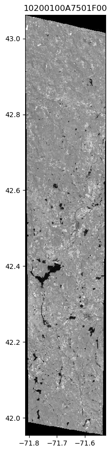
Maxar provides monochrome uint8 or RGB browse images at ~30m resolution that we can visualize before ordering the full-resolution scenes.
# We first convert from geopandas metadata to a pystac items
items = coincident.search.to_pystac_items(gf_stereo)
da = coincident.io.xarray.open_maxar_browse(items[0]).squeeze()
da
<xarray.DataArray 'band_data' (y: 3848, x: 1005)> Size: 4MB
[3867240 values with dtype=uint8]
Coordinates:
    band         int64 8B 1
  * x            (x) float64 8kB -71.81 -71.81 -71.81 ... -71.53 -71.53 -71.53
  * y            (y) float64 31kB 43.06 43.06 43.06 43.06 ... 41.95 41.95 41.95
    spatial_ref  int64 8B ...
Attributes:
    AREA_OR_POINT:  Area
    scale_factor:   1.0
add_offset: 0.0Plot browse image#
For convenience you can create simplified figures directly without first loading the data with Xarray. Browse images are cloud-optimized-geotiffs with overviews for efficient previewing.
coincident.plot.plot_maxar_browse(items[0], overview_level=2);
Advanced Search#
Optical imagery often has estimates of cloud-cover in the metadata. This is typically a single percentage value for the entire scene footprint. The Maxar API goes a step further allowing for filtering cloudcover for only the AOI rather than the entire scene footprint.
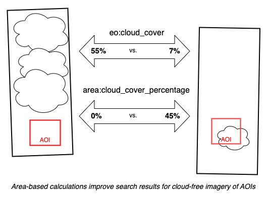
Activating the “area_based_calc” search feature through coincident requires modifying the default “maxar” dataset class. Once activated, in addition to ‘eo:cloud_cover’ ‘view:off_nadir’ metadata will include ‘area:cloud_cover_percentage’ and ‘area:avg_off_nadir_angle’
Note that these searches will take longer!
maxar = coincident.datasets.maxar.Stereo()
maxar
Stereo(alias='maxar', has_stac_api=True, collections=['wv01', 'wv02', 'wv03-vnir', 'ge01'], search='https://api.maxar.com/discovery/v1/search', start='2007-01-01', end=None, type='stereo', provider='maxar', stac_kwargs={'limit': 1000}, area_based_calc=False)
# Use AOI-based estimates of cloud-cover instead of entire scene
maxar.area_based_calc = True
gf = coincident.search.search(
    dataset=maxar,
    bbox=bbox,
    datetime=["2021-03-08", "2021-04-01"],
)

cols = [
    "title",
    "eo:cloud_cover",
    "area:cloud_cover_percentage",
    "view:off_nadir",
    "area:avg_off_nadir_angle",
]
gf[cols]
| title | eo:cloud_cover | area:cloud_cover_percentage | view:off_nadir | area:avg_off_nadir_angle | |
|---|---|---|---|---|---|
| 1 | Maxar WV03 Image 104001006724D500 | 51.883057 | 56.321858 | 28.113903 | 27.457075 |
| 2 | Maxar WV03 Image 1040010067B67700 | 53.269228 | 56.163321 | 27.786872 | 27.291414 |
| 4 | Maxar WV01 Image 10200100A7501F00 | 0.030452 | 0.106177 | 31.826101 | 29.858223 |
| 5 | Maxar WV01 Image 10200100A7DB4600 | 0.008860 | 0.029973 | 27.381504 | 27.601220 |
| 6 | Maxar WV02 Image 10300100BB606C00 | 99.929227 | 99.509544 | 29.767852 | 28.523544 |
| 7 | Maxar WV02 Image 10300100BB8EC300 | 99.952654 | 99.686856 | 24.006449 | 23.991434 |
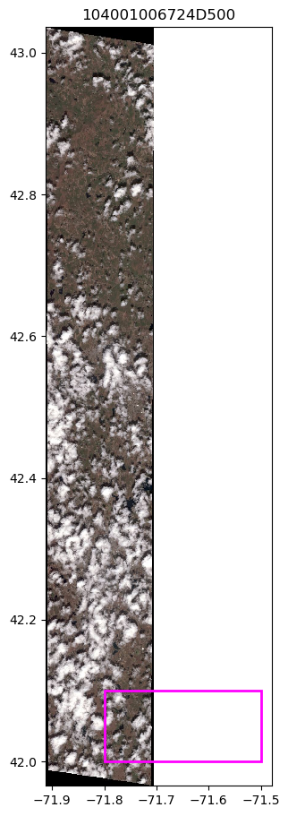
# Plot with cloud-cover
items = coincident.search.to_pystac_items(gf)
item = items[0]

ax = coincident.plot.plot_maxar_browse(item, overview_level=1)
# Add AOI
rect = plt.Rectangle(
    (bbox[0], bbox[1]),
    bbox[2] - bbox[0],
    bbox[3] - bbox[1],
    linewidth=2,
    edgecolor="magenta",
    facecolor="none",
)
ax.add_patch(rect)
plt.autoscale()
Load cloud-cover polygon#
For each acquisition, Maxar includes a Multipolygon that estimates cloud cover. Behind the scenes, coincident uses the stac-asset library to read and download assets of any STAC item. Because stac-asset uses asynchronous functions, you have to use await to return results.
bytes = await coincident.io.download.read_href(item, "cloud-cover")
gf_clouds = gpd.read_file(bytes)
gf_clouds.explore()
Download browse image + metadata#
coincident wraps the stac-asset library to easily download local copies of a STAC item and all of its assets (e.g. metadata and cloud cover mask)
# Set download directory to match item STAC ID
download_dir = f"/tmp/{item.id}"
local_item = await coincident.io.download.download_item(item, download_dir)
/home/docs/checkouts/readthedocs.org/user_builds/coincident/checkouts/104/.pixi/envs/dev/lib/python3.12/site-packages/stac_asset/http_client.py:177: UserWarning: the actual content type does not match the expected: actual=application/json, expected=application/geo+json
  warnings.warn(str(err))
!ls {download_dir}
104001006724D500.browse.tif  104001006724D500.json
104001006724D500.cloud.json  104001006724D500.sample-points.json