Sliderule data I/O

This notebook will highlight analyzing various coincident elevation measurements. We will find regions with and use slideruleearth.io service to retrieve ICESat-2 and GEDI point elevation measurements.

Note

Keep in mind, these measurements are from different sensor types, close in time, but not at exactly the same time. All measurements also have uncertainties, so we do not expect perfect agreement.

import coincident
from mpl_toolkits.axes_grid1.inset_locator import inset_axes
import matplotlib.pyplot as plt
import numpy as np

# For testing
# import sliderule
# sliderule.init(url='slideruleearth.io', verbose=True)

/home/docs/checkouts/readthedocs.org/user_builds/coincident/checkouts/104/src/coincident/io/download.py:27: TqdmExperimentalWarning: Using `tqdm.autonotebook.tqdm` in notebook mode. Use `tqdm.tqdm` instead to force console mode (e.g. in jupyter console)
  from tqdm.autonotebook import tqdm

%matplotlib inline
# %config InlineBackend.figure_format = 'retina'

Identify a primary dataset

Start by loading a full resolution polygon of a 3DEP LiDAR workunit which has a known start_datetime and end_datatime:

workunit = "CO_WestCentral_2019"
df_wesm = coincident.search.wesm.read_wesm_csv()
gf_lidar = coincident.search.wesm.load_by_fid(
    df_wesm[df_wesm.workunit == workunit].index
)
gf_lidar

	workunit	workunit_id	project	project_id	start_datetime	end_datetime	ql	spec	p_method	dem_gsd_meters	...	seamless_category	seamless_reason	lpc_link	sourcedem_link	metadata_link	geometry	collection	datetime	dayofyear	duration
0	CO_WestCentral_2019	175984	CO_WestCentral_2019_A19	175987	2019-08-21	2019-09-19	QL 2	USGS Lidar Base Specification 1.3	linear-mode lidar	1.0	...	Meets	Meets 3DEP seamless DEM requirements	https://rockyweb.usgs.gov/vdelivery/Datasets/S...	http://prd-tnm.s3.amazonaws.com/index.html?pre...	http://prd-tnm.s3.amazonaws.com/index.html?pre...	MULTIPOLYGON (((-106.17143 38.42061, -106.3208...	3DEP	2019-09-04 12:00:00	247	29

1 rows × 33 columns

Search secondary datasets

Provide a list that will be searched in order. The list contains tuples of dataset aliases and the temporal pad in days to search before the primary dataset start and end dates

secondary_datasets = [
    ("gedi", 40),  # +/- 40 days from lidar
    ("icesat-2", 60),  # +/- 60 days from lidar
]

gf_gedi, gf_is2 = coincident.search.cascading_search(
    gf_lidar,
    secondary_datasets,
    min_overlap_area=30,  # km^2
)

Get ICESat-2 ATL06 Data

We’ve identified 7 granules of icesat-2 data to examine, but there is no need to work with the entire granule, which spans a huge geographic extent. Instead we’ll retrieve a subset of elevation values in the area of interest for each granule.

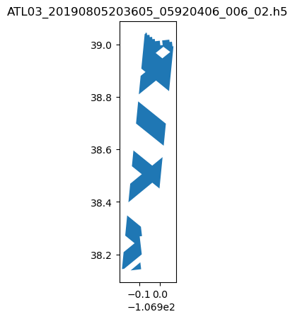
# Hone in on single granule as a pandas series
i = 0
granule_gdf = gf_is2.iloc[[i]]
granule = gf_is2.iloc[i]
granule_gdf.plot()  # needs to be a geodataframe
plt.title(granule.id);
# The icesat-2 track trends N-S, and is crossed by multiple GEDI tracks, resulting in the crosshatched appearance

data_is2 = coincident.io.sliderule.subset_atl06(
    granule_gdf,
    include_worldcover=True,
)

# Plot this data and overlay footprint
fig, ax = plt.subplots(figsize=(8, 10))
plt.scatter(
    x=data_is2.geometry.x,
    y=data_is2.geometry.y,
    c=data_is2.h_li,
    s=10,
)
granule_gdf.dissolve().boundary.plot(ax=ax, color="magenta")
cb = plt.colorbar()
cb.set_label("elevation_hr (m)")

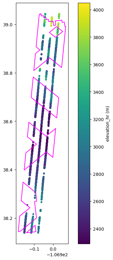
Note

sliderule gets data from the envelope of multipolygon, not only data within intersecting GEDI tracks. Along-track gaps are where there is missing data.

# Here, we specify aoi=granule_gdf to only return GEDI data
# in our icesat-2 track of interest
data_gedi = coincident.io.sliderule.subset_gedi02a(
    gf_gedi,
    aoi=granule_gdf,
    include_worldcover=True,
)

data_gedi

	solar_elevation	flags	sensitivity	elevation_hr	elevation_lm	beam	track	orbit	geometry	worldcover.time	worldcover.value	worldcover.flags	worldcover.file_id
time
2019-09-23 08:03:40.028272128	-48.950699	130	0.915599	2970.799561	2964.996582	2	480	4416	POINT (-107.05912 38.62987)	1.309046e+09	Tree cover	0.0	4.724464e+10
2019-09-23 08:03:40.065466880	-48.957371	130	0.935781	3084.797852	3060.687012	3	480	4416	POINT (-107.05798 38.62212)	1.309046e+09	Tree cover	0.0	4.724464e+10
2019-09-23 08:03:40.148106752	-48.958637	130	0.900905	3043.598877	3021.360107	3	480	4416	POINT (-107.0529 38.61885)	1.309046e+09	Tree cover	0.0	4.724464e+10
2019-09-23 08:03:40.164634624	-48.958889	130	0.906498	3023.866211	3002.188965	3	480	4416	POINT (-107.05188 38.6182)	1.309046e+09	Tree cover	0.0	4.724464e+10
2019-09-23 08:03:40.164634624	-48.960491	130	0.905244	2792.681885	2769.727051	5	480	4416	POINT (-107.07904 38.62588)	1.309046e+09	Tree cover	0.0	4.724464e+10
...	...	...	...	...	...	...	...	...	...	...	...	...	...
2019-10-27 11:45:12.254580224	-21.202047	130	0.960664	3284.958740	3254.115967	11	2006	4946	POINT (-107.06034 39.0425)	1.309046e+09	Tree cover	0.0	8.160438e+10
2019-10-27 11:45:12.262844416	-21.201624	130	0.962776	3294.617432	3278.242676	11	2006	4946	POINT (-107.05984 39.04281)	1.309046e+09	Grassland	0.0	8.160438e+10
2019-10-27 11:45:12.271110400	-21.201200	130	0.967792	3308.820557	3302.016357	11	2006	4946	POINT (-107.05934 39.04312)	1.309046e+09	Grassland	0.0	8.160438e+10
2019-10-27 11:45:12.279376384	-21.200781	130	0.909410	3327.383057	3322.971680	11	2006	4946	POINT (-107.05884 39.04343)	1.309046e+09	Grassland	0.0	8.160438e+10
2019-10-27 11:45:12.287642368	-21.200354	130	0.972252	3328.869141	3320.681641	11	2006	4946	POINT (-107.05832 39.04376)	NaN	NaN	NaN	NaN

7195 rows × 13 columns

# Plot this data and overlay footprint
fig, ax = plt.subplots(figsize=(8, 10))
plt.scatter(
    x=data_gedi.geometry.x,
    y=data_gedi.geometry.y,
    c=data_gedi.elevation_hr,
    s=10,
)
granule_gdf.dissolve().boundary.plot(ax=ax, color="magenta")
cb = plt.colorbar()
cb.set_label("elevation_hr (m)")

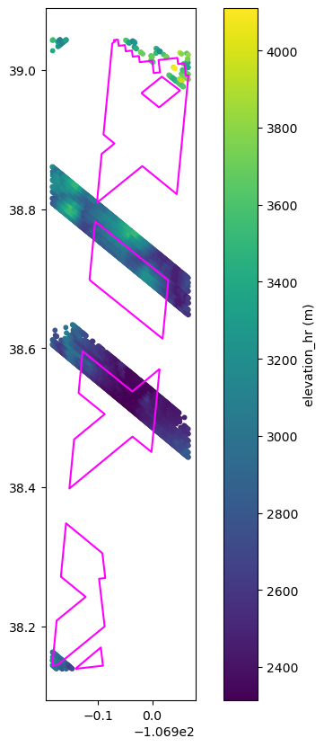
NOTE Like ICESat-2, it’s possible to have points falling outside the estimated footprints

Spatial join: nearest points

NOTE: we will not worry about the difference in time of acquisition between adjacent points for now

utm_crs = granule_gdf.estimate_utm_crs()
data_is2_utm = data_is2.to_crs(utm_crs)
data_gedi_utm = data_gedi.to_crs(utm_crs)

# find nearest IS2 point to each GEDI
close_gedi = data_gedi_utm.sjoin_nearest(
    data_is2_utm,
    how="left",
    max_distance=100,  # at most 100m apart
    distance_col="distances",
)
# index is GEDI subset (with _left added), with _right appended to is2 columns + Distances in meters
close_gedi = close_gedi[close_gedi["distances"].notna()]

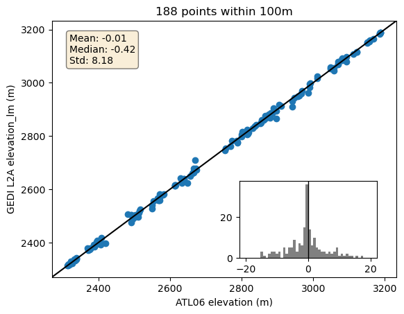
fig, ax = plt.subplots()
plt.scatter(close_gedi.h_li, close_gedi.elevation_lm)
ax.axline((0, 0), slope=1, color="k", transform=ax.transAxes)
plt.xlabel("ATL06 elevation (m)")
plt.ylabel("GEDI L2A elevation_lm (m)")
plt.title(f"{len(close_gedi)} points within 100m")


# Add statistics and inset histogram to plot
inset_ax = inset_axes(ax, width="40%", height="30%", borderpad=2, loc="lower right")


residuals = close_gedi.h_li - close_gedi.elevation_lm
mean_residual = np.mean(residuals)
median_residual = np.median(residuals)
std_residual = np.std(residuals)
textstr = "\n".join(
    (
        f"Mean: {mean_residual:.2f}",
        f"Median: {median_residual:.2f}",
        f"Std: {std_residual:.2f}",
    )
)
props = dict(boxstyle="round", facecolor="wheat", alpha=0.5)
ax.text(
    0.05,
    0.95,
    textstr,
    transform=ax.transAxes,
    fontsize=10,
    verticalalignment="top",
    bbox=props,
)

_ = inset_ax.hist(residuals, bins=50, range=(-20, 20), color="gray")
inset_ax.axvline(0, color="k", linestyle="-", linewidth=1);

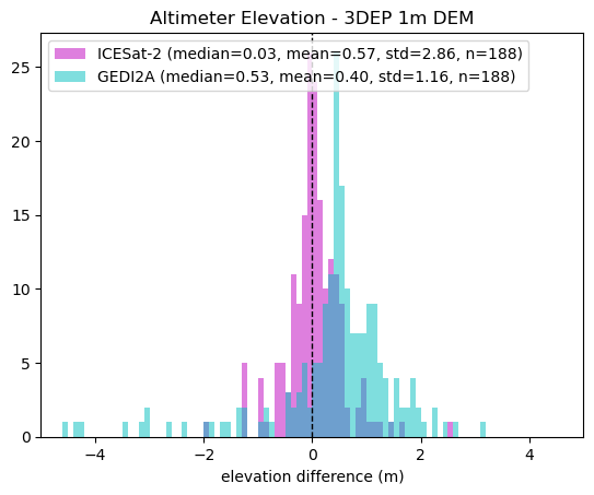
Sample 3DEP

Sample 3DEP 1m DEM at the subset of GEDI Points

Note

SlideRule returns all elevation data in EPSG:7912

close_gedi_3dep = coincident.io.sliderule.sample_3dep(
    close_gedi,
    # Restrict to only DEMs derived from specific WESM LiDAR project
    project_name=gf_lidar["project"].iloc[0],
)

# Add 3DEP elevation values to existing dataframe
close_gedi["elevation_3dep"] = close_gedi_3dep.value.values

# Geometries of nearest IS2 points
close_is2 = data_is2_utm.loc[close_gedi.time_right]

# Sample 3DEP at the subset of GEDI Points
close_is2_3dep = coincident.io.sliderule.sample_3dep(
    close_is2,
    project_name=gf_lidar["project"].iloc[0],
)

close_is2["elevation_3dep"] = close_is2_3dep.value.values

plt.axvline(0, color="k", linestyle="dashed", linewidth=1)

diff_3dep = close_is2.h_li.values - close_is2.elevation_3dep
label = f"ICESat-2 (median={np.nanmedian(diff_3dep):.2f}, mean={np.nanmean(diff_3dep):.2f}, std={np.nanstd(diff_3dep):.2f}, n={len(diff_3dep)})"
plt.hist(diff_3dep, range=[-5, 5], bins=100, color="m", alpha=0.5, label=label)

diff_3dep = close_gedi.elevation_lm.values - close_gedi.elevation_3dep
label = f"GEDI2A (median={np.nanmedian(diff_3dep):.2f}, mean={np.nanmean(diff_3dep):.2f}, std={np.nanstd(diff_3dep):.2f}, n={len(diff_3dep)})"
plt.hist(diff_3dep, range=[-5, 5], bins=100, color="c", alpha=0.5, label=label)

plt.xlabel("elevation difference (m)")
plt.title("Altimeter Elevation - 3DEP 1m DEM")
plt.xlim(-5, 5)
plt.legend(loc="upper left");